Books · The Fiddler: Solutions
Chapter 42
Can You Box the Letters?
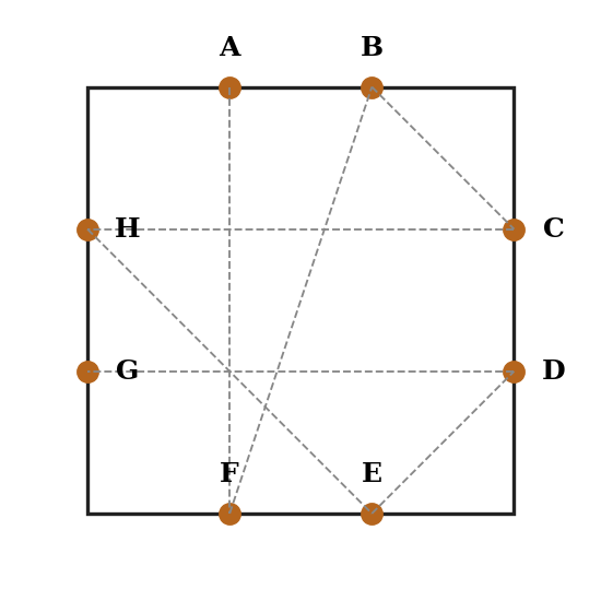
A square has eight points on it, labelled A through H, two on each side. A “letter boxed” sequence visits all eight points, with the rule that two consecutive points in the sequence are never on the same side. (For example AFBCHEDG is valid, while AFBCHGED is not, since H and G share a side.) How many distinct valid sequences use all eight points?
The Fiddler, Zach Wissner-Gross, September 12, 2025(original post)
Solution
Treat each side as a colour, so we are arranging four colours, each appearing twice, with no two equal colours adjacent, and then distinguishing the two points of each colour. The number of colour-patterns with no equal neighbours is, by inclusion–exclusion on which colours are glued together, Each side’s two points are distinct and can be ordered in ways, contributing :
The computation
With only eight points the whole thing is small enough to count head-on: run through all orderings and keep those in which no two consecutive points share a side.
from itertools import permutations
side = dict(zip('ABCDEFGH', [0, 0, 1, 1, 2, 2, 3, 3]))     # two points per side
cnt = sum(all(side[s[i]] != side[s[i+1]] for i in range(7))
          for s in permutations('ABCDEFGH'))
print(cnt)                               # 13824
Extra Credit
Now the square has twelve points, A through L, three on each side, with the same rule. How many valid sequences use all twelve?
Solution
Arrange four colours, each appearing three times, with no two equal adjacent, then order the three points on each side in ways. Counting the no-equal-neighbour colour patterns and multiplying by gives (The source’s count is paywalled; this is my own enumeration.)
The computation
Twelve points make too many to sweep, but the side-pattern is just the distinct arrangements of four colours three-apiece (only ). Count those with no equal neighbours, then multiply by the orderings of each side’s three points.
from sympy.utilities.iterables import multiset_permutations
from math import factorial
pat = sum(all(p[i] != p[i+1] for i in range(11))
          for p in multiset_permutations('AAABBBCCCDDD'))
print(pat, pat * factorial(3)**4)        # 41304  53529984