Ostomachion

More than two thousand years before the four-colour theorem was proved, Archimedes of Syracuse described the Ostomachion: a dissection of a $12 \times 12$ square into fourteen polygonal pieces, together with problems about the distinct ways the pieces can be rearranged to reconstitute the square. The counting problem is a polyomino-packing question in slightly thickened form — pieces are triangles and quadrilaterals rather than unit-cell polyominoes — and was answered by William Cutler in $2003$: the dissection admits exactly $17\,152$ reassemblies, or $536$ modulo the symmetries of the square.

We take a different classical problem here: given the Ostomachion’s fixed dissection, colour the fourteen regions with four colours so that (i) adjacent regions receive different colours, and (ii) each of the four colour classes occupies the same total area, namely $36$ square units. This is a four-colouring of the planar map with an added equal-partition-of-area constraint. It resembles the four-colour theorem in requiring only four colours, but it is a substantially stronger problem: the colour classes must be equal in area, and the equal-area constraint cuts the number of proper colourings down to a mere handful. The exact figure, which we shall establish below, is $9$ distinct colourings up to a permutation of the four colours.

The dissection

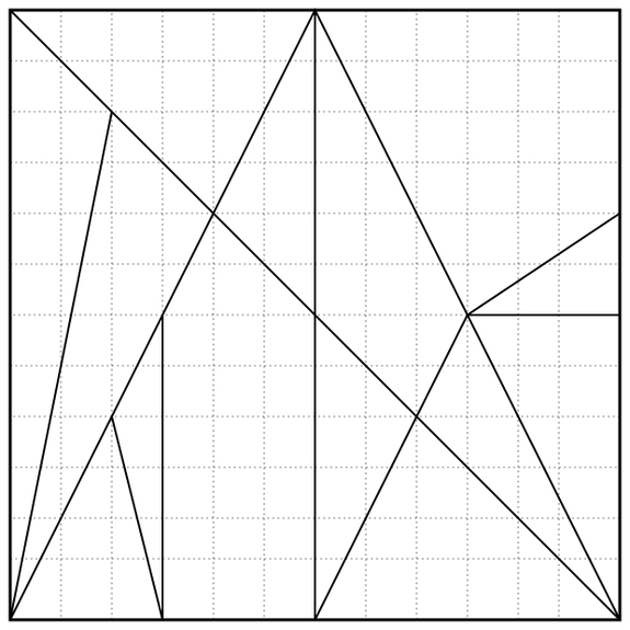
Archimedes’ dissection is shown in Figure 7.1. The fourteen regions are labelled $0$ through $13$; their areas are given (in order) by $$12, \; 6, \; 21, \; 3, \; 6, \; 12, \; 12, \; 24, \; 3, \; 9, \; 6, \; 12, \; 6, \; 12,$$ summing to $144 = 12^2$. The precise vertex coordinates, although historically reconstructed from the Archimedes Palimpsest, are not required here: only the areas and the adjacency graph matter for the colouring problem.

The adjacency graph — two regions are adjacent iff they share a segment of positive length — has $14$ vertices and $20$ edges, shown in Figure 7.2 together with one valid equal-area $4$-colouring.

The programming model

Variables

For each region $i \in \{0, 1, \ldots, 13\}$, introduce an integer variable $X_i \in \{0, 1, 2, 3\}$ representing its colour.

Proper colouring

For every adjacent pair $\{i, j\}$ in the adjacency graph, $$X_i \;\neq\; X_j.$$

Equal areas per colour class

For each colour $c \in \{0, 1, 2, 3\}$, $$\sum_{i = 0}^{13} \mathbb{1}[X_i = c] \cdot a_i \;=\; 36,$$ where $a_i$ is the area of region $i$. In CP-SAT this is encoded by introducing one Boolean indicator $b_{i, c}$ per region-colour pair, setting $b_{i, c} = \mathbb{1}[X_i = c]$ via reified equality, and summing $\sum_i a_i b_{i, c} = 36$.

Colour-permutation symmetry

The problem is symmetric under the $4! = 24$ permutations of the four colours. The simplest way to break this symmetry without losing solutions is to pin the colour of a single region, for example $$X_0 \;=\; 0.$$ Pinning $X_0$ removes one factor of the $4! = 24$ colour permutations, namely the choice of which colour to call colour $0$. What remains is the freedom to relabel the other three colours among themselves, a residual symmetry of $3! = 6$; this is resolved at count time by dividing the enumeration total by $6$.

A solver in forty lines

from ortools.sat.python import cp_model

CONNECT = {
    0: [1, 5, 6],    1: [0, 2, 13],
    2: [1, 12, 3, 5], 3: [2, 4, 5],
    4: [3, 5],       5: [0, 2, 3, 4, 6],
    6: [0, 5],       7: [8, 13],
    8: [7, 9],       9: [8, 10],
    10: [9, 11, 13], 11: [10, 12],
    12: [11, 13, 2], 13: [1, 7, 10, 12],
}
AREAS = [12, 6, 21, 3, 6, 12, 12,
         24, 3, 9, 6, 12, 6, 12]

def solve():
    m = cp_model.CpModel()
    K, n = 4, 14
    x = [m.NewIntVar(0, K - 1, "") for _ in range(n)]
    for i, neigh in CONNECT.items():
        for j in neigh:
            if j > i:
                m.Add(x[i] != x[j])
    target = sum(AREAS) // K
    for c in range(K):
        b = [m.NewBoolVar("") for _ in range(n)]
        for i in range(n):
            m.Add(x[i] == c).OnlyEnforceIf(b[i])
            m.Add(x[i] != c).OnlyEnforceIf(b[i].Not())
        m.Add(sum(AREAS[i] * b[i]
                  for i in range(n)) == target)
    m.Add(x[0] == 0)  # pin one colour to break symmetry
    s = cp_model.CpSolver()
    s.Solve(m)
    return [s.Value(v) for v in x]

The solver returns one equal-area $4$-colouring in about $200$ milliseconds. Enabling enumeration of all feasible models (parameters.enumerate_all_solutions = True) reveals that there are exactly $54$ colourings once the pinning $X_0 = 0$ is imposed. Pinning fixes the colour of region $0$ to one of the four colours, so the $54$ pinned colourings correspond to $54 \times 4 = 216$ raw colourings in total. To count colourings up to a permutation of the four colours, we collapse each orbit of the full $4! = 24$ permutation group; doing so over all $216$ raw colourings leaves exactly $9$ colourings up to permutation. (Pinning a single region does not by itself quotient out the whole symmetry group: the three remaining colours can still be relabelled, so the $54$ figure overcounts the $9$ genuinely distinct colourings.)

Sources. Archimedes’ treatise on the Ostomachion survives in fragmentary form in the Archimedes Palimpsest; Reviel Netz’s edition (The Archimedes Codex, $2007$) contains the reconstructed Greek text and a discussion of the counting problem that evidently interested Archimedes, namely the enumeration of distinct reassemblies. The $17\,152$-solution count (or $536$ up to the dihedral symmetry of the square) is due to William Cutler, communicated informally in $2003$ and independently verified by several authors since. The equal-area $4$-colouring variant used here is a modern exercise, convenient precisely because the fourteen areas $3, 3, 6, 6, 6, 6, 9, 12, 12, 12, 12, 12, 21, 24$ sum to a multiple of $4$; it is unclear whether any ancient author posed it.