Introduction
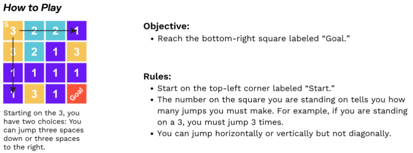
The Jumping Julia Maze from the amazing Julia Robinson Maths Festival is an intriguing puzzle where players must navigate from a starting position to a goal by making jumps based on numbers in a grid. In this post, we’ll break down the problem and implement a solution using Python, NetworkX, and Matplotlib.
Problem Description

Solution Approach
1. Graph Representation
The key insight is to model this as a graph problem:
- Each square in the grid becomes a node.
- Valid jumps become directed edges between nodes.
- Finding a solution becomes a shortest path problem.
Why a graph?
- Natural representation of connected positions.
- Well-established algorithms for path finding.
- Easy visualization capabilities.
2. Implementation Components
a. The JumpingMaze Class
class JumpingMaze:
    def __init__(self, grid):
        self.grid = np.array(grid)
        self.rows, self.cols = self.grid.shape
        self.G = self._create_graph()
b. Graph Creation
The critical part is creating edges for valid jumps:
def _create_graph(self):
    G = nx.DiGraph()

    # Add nodes
    for i in range(self.rows):
        for j in range(self.cols):
            G.add_node((i, j), pos=(j, -i))

    # Add edges for valid jumps
    for i in range(self.rows):
        for j in range(self.cols):
            jumps = self.grid[i, j]
            if jumps == 0:  # Skip goal node
                continue

            # Horizontal jumps
            for dx in [-jumps, jumps]:
                new_j = j + dx
                if 0 <= new_j < self.cols:
                    G.add_edge((i, j), (i, new_j))

            # Vertical jumps
            for dy in [-jumps, jumps]:
                new_i = i + dy
                if 0 <= new_i < self.rows:
                    G.add_edge((i, j), (new_i, j))
Key Points:
- Each node is represented by its (row, col) coordinates.
- Edges are only created for exact jump distances.
- The goal node (0 value) doesn’t need outgoing edges.
3. Finding the Solution
We use NetworkX’s shortest_path algorithm:
def find_solution(self, start=(0, 0)):
    goal = (self.rows - 1, self.cols - 1)
    try:
        return nx.shortest_path(self.G, start, goal)
    except nx.NetworkXNoPath:
        return None
This efficiently finds:
- The shortest sequence of jumps to reach the goal.
- Or determines that no solution exists.
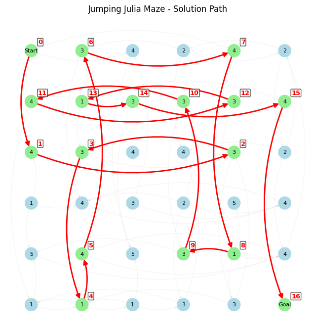
4. Visualizing the solution
Our visualization includes several key features:
Node colors:
- Light blue for regular squares.
- Light green for squares in the solution path.
Arrows:
- Gray curved arrows for all possible jumps.
- Bold red curved arrows for the solution path.
Labels:
- Grid numbers in each square.
- Sequential numbers for solution steps.
- Special labels for Start and Goal.
How to Use the Solution
- Create your grid:
grid = [
    [3, 2, 2, 1],
    [3, 2, 1, 3],
    [1, 1, 1, 1],
    [1, 3, 1, 0]
]
- Initialize the maze:
maze = JumpingMaze(grid)
- Find and visualize the solution:
path = maze.find_solution()
if path:
    maze.visualize(path)
else:
    print("No solution exists!")
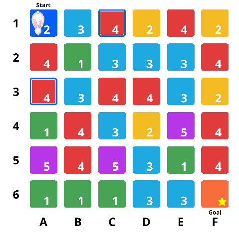
A hard maze example
Here is a hard maze along with the solution:


Conclusion
The Jumping Julia Maze demonstrates how graph theory can elegantly solve path-finding puzzles. By converting the grid into a graph, we can leverage existing algorithms to find solutions efficiently and create clear visualizations to understand the path.