A Faulty Traffic Signal

Problem

A faulty traffic signal has a 15-second cycle of Red and Green (no Orange). In each cycle, the Red time ($R$) is uniformly distributed between 0 to 15 seconds, and the remaining time ($15 - R$) is Green. You arrive at a completely random time. If it’s Green, you cross immediately, with your crossing time uniformly distributed over the remaining Green time left. If it’s Red, you wait for Green and then cross, with your crossing time uniformly distributed over the total Green time of that cycle. Find $\mathbb{P}(\text{Red})$, $\mathbb{P}(\text{Green})$, $\mathbb{E}(\text{Waiting time} \mid \text{Red arrival})$, and $\mathbb{E}(\text{Total time to cross})$?

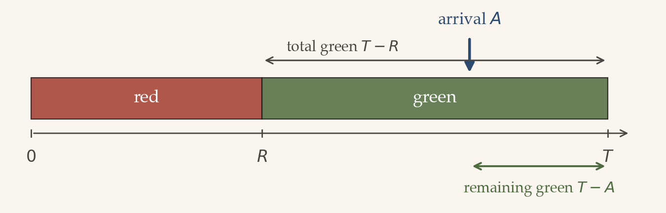
Throughout, write $T = 15$ for the period. Put the red phase at the start of each cycle, on $[0, R)$, and the green phase at the end, on $[R, T)$; the answer cannot depend on this choice. Let $A$ be the arrival time, uniform on $(0, T)$ and independent of $R$. Then you meet red exactly when $A < R$.

The chance of red, and the chance of green

Both random choices, the split $R$ and the arrival $A$, are uniform and independent, so the pair $(R, A)$ is spread evenly over the square $[0, T]^2$. You meet red exactly when $A < R$, the triangle below the diagonal; you meet green when $A > R$, the triangle above it. The diagonal cuts the square into two equal halves, so $\mathbb{P}(\text{red}) = \mathbb{P}(\text{green}) = \tfrac12,$ with no calculation at all.

If you prefer the integral, the same answer falls out. For a fixed split $R = r$, red fills a fraction $r/T$ of the cycle, so $\mathbb{P}(\text{red}\mid R = r) = r/T$. Averaging over the uniform split, whose density is $1/T$, $\mathbb{P}(\text{red}) = \int_0^T \frac{r}{T}\cdot\frac{1}{T}\,dr = \frac{1}{T^2}\cdot\frac{T^2}{2} = \frac12.$ The split averages out: a single cycle is lopsided, but over many cycles a red second is as likely as a green one, because the average red, $\mathbb{E}[R] = T/2$, sits exactly in the middle.

A red light means the red was probably long

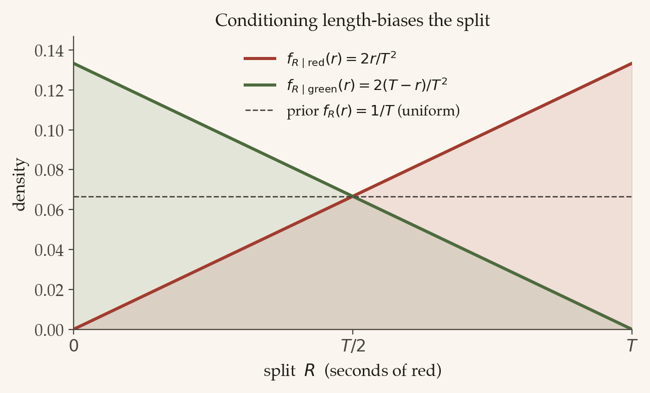
To average the wait we need the distribution of the split among the cycles where we actually hit red, and that is not the plain uniform split. A long red covers more of the cycle, so it is more likely to be the one you walk into; learning that you met red therefore makes long reds more likely. This effect is known as length-biasing.

We can read the corrected density straight off the cycle. The chance of both meeting red and having a split near $r$ is $(r/T)(1/T)\,dr$. Dividing by the overall chance of red, $\tfrac12$, gives the density of the split among red arrivals, $f_{R\mid\text{red}}(r) = \frac{(r/T)(1/T)}{1/2} = \frac{2r}{T^2}, \qquad 0 < r < T.$ It rises with $r$, and it integrates to one. The same reasoning for green gives a density that falls, $f_{R\mid\text{green}}(r) = \frac{2(T - r)}{T^2}, \qquad 0 < r < T.$

How long you wait at a red light

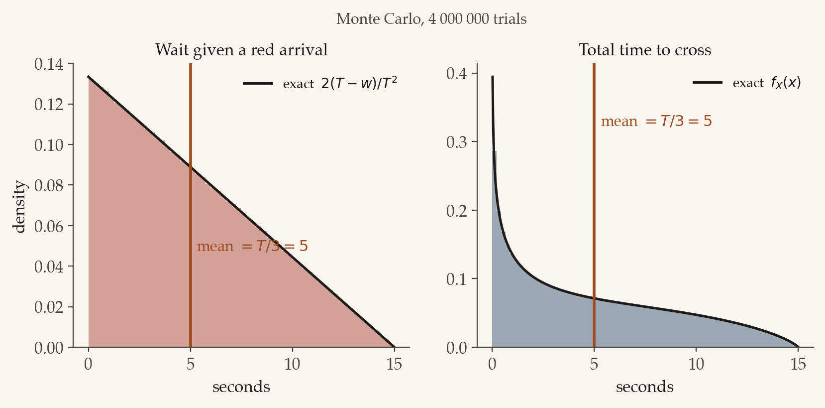
Arrive on red with split $R = r$. Your arrival is equally likely anywhere in the red, so the red still to come is uniform on $(0, r)$, with average $r/2$. Averaging this over the red-arrival density, $\mathbb{E}[\,W \mid \text{red}\,] = \int_0^T \frac{r}{2}\cdot\frac{2r}{T^2}\,dr = \frac{1}{T^2}\int_0^T r^2\,dr = \frac{1}{T^2}\cdot\frac{T^3}{3} = \frac{T}{3}.$ With $T = 15$ the expected wait is 5 seconds.

The value $T/3$ is larger than a first guess suggests. Averaging the red to $T/2$ and halving it for the uniform wait would give $T/4$, but this overlooks the length-biasing: longer reds are met more often and carry longer waits, so the average comes to $T/3$ rather than $T/4$.

How long the crossing takes

If you arrived on red, the whole of the green phase still lies ahead, so your crossing is spread over all of it, $(0, T - r)$, with average $(T - r)/2$. Against the red-arrival density, $\mathbb{E}[\,C \mid \text{red}\,] = \int_0^T \frac{T - r}{2}\cdot\frac{2r}{T^2}\,dr = \frac{1}{T^2}\int_0^T r(T - r)\,dr = \frac{1}{T^2}\cdot\frac{T^3}{6} = \frac{T}{6}.$

If you arrived on green, two quantities are random at once. The green still showing when you arrive is some fraction of the full green, and your crossing then takes some fraction of that. Each fraction is uniform between zero and the whole, so each averages a half, and a half of a half is a quarter: $\mathbb{E}[\,C \mid \text{green},\ R = r\,] = \tfrac12\cdot\tfrac12\,(T - r) = \frac{T - r}{4}.$ Averaging over the green-arrival density, $\mathbb{E}[\,C \mid \text{green}\,] = \int_0^T \frac{T - r}{4}\cdot\frac{2(T - r)}{T^2}\,dr = \frac{1}{2T^2}\int_0^T (T - r)^2\,dr = \frac{1}{2T^2}\cdot\frac{T^3}{3} = \frac{T}{6}.$

So the expected crossing is $T/6 = 2.5$ seconds either way. That the two cases agree is a small coincidence: arriving on red favours short greens, pulling the crossing down, while arriving on green halves the remaining green a second time, and the two pulls happen to cancel.

The total time to cross

The total time is the wait plus the crossing, and the wait is zero unless you arrived on red. Weighing the two cases by their equal probabilities,

$$\begin{aligned} \mathbb{E}[\,\text{total}\,] &= \tfrac12\bigl(\mathbb{E}[W\mid\text{red}] + \mathbb{E}[C\mid\text{red}]\bigr) + \tfrac12\,\mathbb{E}[C\mid\text{green}] \\ &= \tfrac12\left(\frac{T}{3} + \frac{T}{6}\right) + \tfrac12\cdot\frac{T}{6} = \frac{T}{4} + \frac{T}{12} = \frac{T}{3}. \end{aligned}$$

With $T = 15$ the expected total time to cross is 5 seconds, the same as the red-light wait on its own. There is no hidden reason for the match; the fractions $\tfrac12(\tfrac13 + \tfrac16) + \tfrac12\cdot\tfrac16$ simply add back to $\tfrac13$.

The same answers, from one diagram

Every mean above can be read straight off a picture, with no integral at all. Redraw the sample square with the arrival time $A$ along the bottom and the red duration $R$ up the side, so each equally likely scenario is a point spread uniformly over $[0, T]^2$. The line $R = A$ splits it: above the line the red outlasts your arrival and you meet red, below it you meet green.

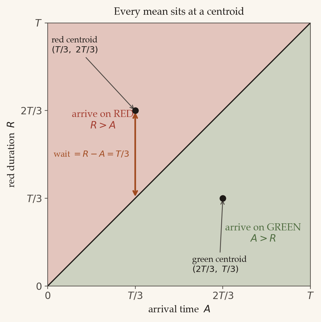
Two facts do all the work. First, the diagonal cuts the square into two equal triangles, so $\mathbb{P}(\text{red}) = \mathbb{P}(\text{green}) = \tfrac12$ by inspection. Second, a quantity that varies linearly across the plane has, as its average over any triangle, simply its value at the triangle’s centroid. This holds because the centroid is the mean position of a point dropped uniformly in the triangle, and it sits at the average of the three corners. The red triangle has corners $(0, 0)$, $(0, T)$, $(T, T)$, so its centroid lies at $(A, R) = (T/3,\, 2T/3)$; the green triangle has corners $(0, 0)$, $(T, 0)$, $(T, T)$, with centroid $(2T/3,\, T/3)$.

Now read each quantity off at the relevant centroid.

• The wait on red is $R - A$, the vertical drop from the point down to the diagonal. At the red centroid this is $2T/3 - T/3 = T/3$.
• The crossing brings in the one ingredient the square cannot show: you cross over a uniform fraction of the green available, which contributes a clean factor of one half. On red the green available is all of it, $T - R$, so the crossing averages $\tfrac12(T - R)$, worth $\tfrac12(T - 2T/3) = T/6$ at the red centroid. On green the green available is the part still showing, $T - A$, so the crossing averages $\tfrac12(T - A)$, worth $\tfrac12(T - 2T/3) = T/6$ at the green centroid.
• The total is the wait plus the crossing, weighted by the two equal halves: $\tfrac12(T/3 + T/6) + \tfrac12\cdot T/6 = T/3$.

All four required answers, $\tfrac12$, $\tfrac12$, $T/3$ and $T/3$, fall out of two centroids and a single factor of a half. The integrals above were never strictly needed for the means; only the full distribution of the total time, derived next, genuinely calls for calculus.

The shape of the total time

The mean is only a summary; the same rules fix the whole spread of the crossing time, and the simulation at the end traces it out. It is worth deriving, both as a check on that plot and because the answer is tidier than the set-up suggests. Measure time as a fraction of the period: put $S = X/T$, where $X$ is the total time. Then $S$ lives on $(0, 1)$, and the density of $X$ itself is recovered by $f_X(x) = \tfrac1T f_S(x/T)$. Take $T = 1$ for the working below. The two arrival types build $S$ differently, so we treat them apart and add.

A green arrival. You cross at once, over a uniform fraction of the green still showing. Fix the arrival at $A = a$: this is a green arrival exactly when the split fell below it, which carries probability $a$, and the crossing is then uniform on $(0, 1 - a)$ with density $1/(1 - a)$. A total of size $s$ needs $1 - a > s$, that is $a < 1 - s$, so the green contribution to the density is $g_{\text{green}}(s) = \int_0^{1-s} a\cdot\frac{1}{1 - a}\,da = \bigl[-a - \ln(1 - a)\bigr]_0^{1-s} = (s - 1) - \ln s.$

A red arrival. Now the total is the wait plus the crossing, $S = W + C$. Fix the split at $R = r$: this is a red arrival with probability $r$, and given it, the wait $W$ is uniform on $(0, r)$ while the crossing $C$ is uniform on $(0, 1 - r)$, the two independent. Their two lengths add to the whole period, so their sum has the trapezoidal density of a convolution, $h_r(s) = \frac{\ell(r, s)}{r(1 - r)}, \qquad \ell(r, s) = \min(1 - r,\, s) - \max(0,\, s - r),$ where $\ell$ is the length of overlap, taken as zero when this is negative. Weighting by the red-arrival probability $r$ cancels the $r$ in the denominator, which is what keeps the answer clean: $g_{\text{red}}(s) = \int_0^1 r\,h_r(s)\,dr = \int_0^1 \frac{\ell(r, s)}{1 - r}\,dr.$ The overlap is piecewise linear in $r$: it equals $r$ for $r < \min(s, 1 - s)$, holds at $\min(s, 1 - s)$ between the two break points, and equals $1 - r$ for $r > \max(s, 1 - s)$. Carrying out the three pieces, the integral collapses to the binary entropy, $g_{\text{red}}(s) = -\,s \ln s - (1 - s)\ln(1 - s).$

Adding the two contributions, $f_S(s) = g_{\text{red}}(s) + g_{\text{green}}(s) = (s - 1)\ln(1 - s) - (s + 1)\ln s + (s - 1), \qquad 0 < s < 1.$ This integrates to one, and $\int_0^1 s\,f_S(s)\,ds = \tfrac13$, which returns the mean $\mathbb{E}[X] = T/3$ found above. The density runs to infinity as $s \to 0$, but only as slowly as $-\ln s$: most crossings are nearly instant, either a green arrival late in a long green, or a red arrival with little red left. At the other end it falls to zero as $s \to 1$, since using almost the whole period needs both a near-full wait and a near-full crossing, which is vanishingly rare. The curve, scaled back to seconds by $f_X(x) = \tfrac1T f_S(x/T)$, is the one drawn over the simulated histogram below.

Quantity	Closed form	Value at $T = 15$
$\mathbb{P}(\text{red})$	$1/2$	$0.5$
$\mathbb{P}(\text{green})$	$1/2$	$0.5$
$\mathbb{E}[\,W \mid \text{red}\,]$	$T/3$	$5.0$ s
$\mathbb{E}[\,C \mid \text{red}\,]$	$T/6$	$2.5$ s
$\mathbb{E}[\,C \mid \text{green}\,]$	$T/6$	$2.5$ s
$\mathbb{E}[\,\text{total time to cross}\,]$	$T/3$	$5.0$ s

Computational verification

We confirm every closed form with a direct simulation. Each trial draws a fresh split $R$ and a fresh arrival $A$, classifies the arrival, and times the wait and the crossing by the rules above. With fifty million trials the Monte Carlo estimates agree with the exact values to three decimal places.

import numpy as np

rng = np.random.default_rng(20260529)
N, T = 50_000_000, 15.0

R = rng.uniform(0, T, N)        # red duration ~ U(0,T); green = T-R
A = rng.uniform(0, T, N)        # arrival uniform within the cycle
is_red = A < R

# probabilities
print(is_red.mean(), (~is_red).mean())          # -> 0.5, 0.5

# waiting time: red -> remaining red R-A; green -> 0
wait = np.where(is_red, R - A, 0.0)
print(wait[is_red].mean())                       # E[W | red]   -> T/3 = 5.0

# crossing time: red over full green (T-R); green over remaining green (T-A)
u = rng.uniform(0, 1, N)
cross = np.where(is_red, u * (T - R), u * (T - A))
print(cross[is_red].mean(), cross[~is_red].mean())  # both -> T/6 = 2.5

print((wait + cross).mean())                     # E[total]     -> T/3 = 5.0

Quantity	Exact	Monte Carlo
$\mathbb{P}(\text{red})$	$0.500$	$0.50010$
$\mathbb{P}(\text{green})$	$0.500$	$0.49990$
$\mathbb{E}[\,W \mid \text{red}\,]$	$5.000$	$5.00071$
$\mathbb{E}[\,C \mid \text{red}\,]$	$2.500$	$2.49988$
$\mathbb{E}[\,C \mid \text{green}\,]$	$2.500$	$2.49992$
$\mathbb{E}[\,\text{total}\,]$	$5.000$	$5.00075$