Problem (Credit: R Muthu Veerappan)
If we pick a random point from a regular polygon, what will be the expected distance of the point from the centre assuming that the circumradius of the polygon is \(1\)?
Solution
Choosing random points in a triangle
To compute the expected distance, using symmetry it is easy to see that we only need to consider the points in a right angled triangle triangle with one vertex at the centre of the regular polygon, one vertex coinciding with the vertex of the polygon and the other one at the midpoint of the edge of the polygon.
If \((0,0)\) is the centre of the regular polygon and the circumradius is one unit, we can always orient the polygon so that the right angled triangle that we wish to draw the random points from have the vertices \((0,0), (\cos(\frac{\pi}{n}),0)\) and \((\cos(\frac{\pi}{n}),\sin(\frac{\pi}{n})).\)
In the figure below, when the regular polygon is an equilateral triangle, we draw the random points from \(\Delta AEC\).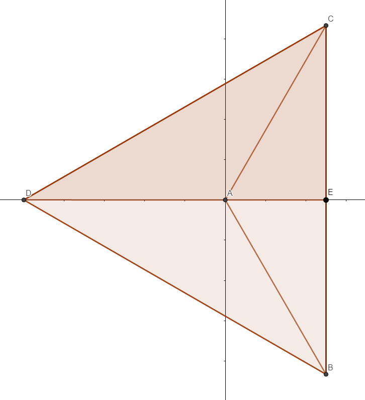
Analytical computation of expected value
We need to evaluate the integral
\[ \int_0^{\cos(\frac{\pi}{n})} \int_0^{x\tan(\frac{\pi}{n})} \sqrt{x^2+y^2} \frac{2}{\sin(\frac{\pi}{n})\cos(\frac{\pi}{n})} dx dy \]
For the substitution, \(x=u\) and \(y=uv\), the Jacobian is given by
\[ \Vert J \Vert = \begin{vmatrix} \frac{\partial x}{\partial u} & \frac{\partial x}{\partial v}\\ \frac{\partial y}{\partial u} & \frac{\partial y}{\partial v} \end{vmatrix} = \begin{vmatrix} 1 & 0 \\ v & u \end{vmatrix} = u \]
The above integral reduces to
\[ \begin{align*} &\frac{2}{\sin(\frac{\pi}{n})\cos(\frac{\pi}{n})}\int_0^{\cos(\frac{\pi}{n})} \int_0^{\tan(\frac{\pi}{n})} u\sqrt{v^2+1} u du dv \\ &=\frac{2}{\sin(\frac{\pi}{n})\cos(\frac{\pi}{n})}\int_0^{\cos(\frac{\pi}{n})} u^2 du \int_0^{\tan(\frac{\pi}{n})} \sqrt{v^2+1} dv \\ &= \frac{\cos^2(\frac{\pi}{n})}{3 \sin (\frac{\pi}{n})}\left(\tan \left(\frac{\pi}{n}\right)\sec \left(\frac{\pi}{n}\right) + \ln\left(\tan\left(\frac{\pi}{n}\right) + \sec\left(\frac{\pi}{n}\right)\right)\right)\\ &=\frac{1}{3} + \frac{\cos^2(\frac{\pi}{n})}{3 \sin (\frac{\pi}{n})}\ln\left(\tan\left(\frac{\pi}{n}\right) + \sec\left(\frac{\pi}{n}\right)\right) \end{align*} \\ \]
The following result which can be easily obtained by using integration by parts was used in the evaluation of the above integral
\[ \int \sqrt{v^2+1} dv = \frac{v\sqrt{v^2+1}}{2} + \frac{1}{2}\ln|v + \sqrt{v^2+1}| + C \]
For \(n=3\), the expected value is given by \(\frac{1}{3} + \frac{\ln(\sqrt{3}+2)}{6\sqrt{3}} = \bf{0.460}\).
For \(n=4\), the expected value is given by \(\frac{1}{3} + \frac{\ln(1+\sqrt{2})}{3\sqrt{2}} = \bf{0.541}\).
Computational Verification
Randomly choosing points in a triangle
There are three well known methods to allow one to uniformly random sample from a triangle. These are:
- The Parallelogram method
- The Kraemer Method
- Inverse cumulative distribution method
The Parallelogram method
The parallelogram method is as follows. 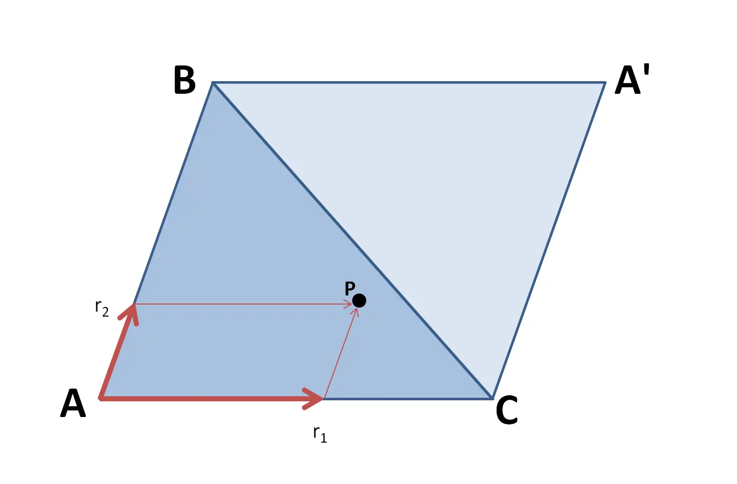
For a triangle \(\Delta ABC\), consider the parallelogram \(ABCA'\).
For a point in the unit square \((r_1,r_2)\), define the point \(P\) such that \(P=r_1 \overline{AC} + r_2\overline{AB}\).
This point will always fall inside the parallelogram. However, if it occurs in the complementary triangle \(BCA'\), then we can either reject the point or reflect it back into the triangle \(ABC\). That is if \(r_1 + r_2 <1\), then \(P=r_1 \overline{AC} + r_2\overline{AB}\), but if \(r_1+r_2>1\), then \(P=(1-r_1)\overline{AC} + (1-r_2)\overline{AB}\).
Kraemer Method
Suppose we have an arbitrary triangle with vertices \(A\), \(B\), and \(C\). In this method, we choose two random numbers in \([0,1]\), \(s\) and \(t\). Let \(t>s\), the point \(sA + (t-s)B + (1-t)C\) is a random point within the triangle \(\Delta ABC\).
Here is a plot of the random points obtained in an equilateral triangle whose median lies on the \(x\)-axis.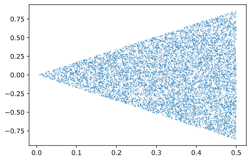
Inverse cumulative distribution method
Suppose we have an arbitrary triangle with vertices \(A\), \(B\), and \(C\). In this method, we choose two random numbers \(r_1\) and \(r_2\) in \([0,1]\) and a point \(P\) such that \(P=(1−\sqrt{r_1})A+\sqrt{r_1}(1−r_2)B+\sqrt{r_1}r_2C\).
\(P\) is a random point within the triangle \(\Delta ABC\).Intuitively, \(\sqrt{r_1}\) sets the percentage from vertex \(A\) to the opposing edge, while \(r_2\) represents the percentage along that edge. Taking the square-root of \(r_1\) gives a uniform random point with respect to surface area. 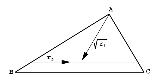
Python code to calculate expected distance
import numpy as np
from math import sqrt

import numpy as np
from math import sqrt

def kraemer_points_on_triangle(v, n):
    x = np.sort(np.random.rand(2, n), axis=0)
    return np.column_stack([x[0], x[1]-x[0], 1.0-x[1]]) @ v

runs = 1000000

#n=3
v = np.array([(0, 0), (0.5, 0), (0.5, sqrt(3)/2)])
points = kraemer_points_on_triangle(v, runs)
print(np.mean(np.sqrt(np.square(points).sum(axis=1))))

#n=4
v = np.array([(0, 0), (0,1/sqrt(2)), (1/sqrt(2), 1/sqrt(2))])
points = kraemer_points_on_triangle(v, runs)
print(np.mean(np.sqrt(np.square(points).sum(axis=1))))
As expected, the expected value from the simulation matches the result that was calculated analytically 😊.