Can you catch the cricket?

Riddler Express

Help, there’s a cricket on my floor! I want to trap it with a cup so that I can safely move it outside. But every time I get close, it hops exactly $1$ foot in a random direction.

I take note of its starting position and come closer. Boom — it hops in a random direction. I get close again. Boom — it takes another hop in a random direction, independent of the direction of the first hop.

What is the most probable distance between the cricket’s current position after two random jumps and its starting position? (Note: This puzzle is not asking for the expected distance, but rather the most probable distance. In other words, if you consider the probability distribution over all possible distances, where is the peak of this distribution?)

Solution

Let $θ$ be the angle between the cricket’s jumps. Using the cosine law, we see that the distance from the center to the end point of the second hop is $\sqrt{2-2\cos\theta}$. The least distance from the starting point is $0$ and the maximum distance is $2$. We can asssume that $θ \sim \mathcal{U}[0, π]$.

For any real $x ∈ [0, 2]$, we have the CDF of $X = \sqrt{2-2\cos\theta}$,

Taking the derivative of the CDF, the PDF of $X$ is $f(x) = \frac{2}{\pi\sqrt{4-x^2}}$ on $[0, 2]$.

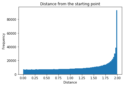
The PDF approaches infinity as $x \rightarrow 2$, therefore the most probable distance is $\textbf{2}$ feet.

Computational solution

From the histogram below, we see that the most probable distance is indeed $\textbf{2}$ feet.

import numpy as np
from math import pi, sqrt, sin, cos
import matplotlib.pyplot as plt

def distances(num_samples = 1000000):
    def dist(row):
        return sqrt((cos(row[0])-cos(row[1]))**2 + (sin(row[0])-sin(row[1]))**2)
    angles = np.random.uniform(0, 2*pi, (num_samples,2))
    return np.apply_along_axis(dist, 1, angles)

def plot_dist_hist(distances):
    plt.hist(distances, bins='auto')
    plt.xlabel('Distance')
    plt.ylabel('Frequency')
    plt.title('Distance from the starting point')

plot_dist_hist(distances())

Riddler Classic

When you roll a pair of fair dice, the most likely outcome is $7$ (which occurs 1/6 of the time) and the least likely outcomes are $2$ and $12$ (which each occur $1/36$ of the time).

Annoyed by the variance of these probabilities, I set out to create a pair of “uniform dice.” These dice still have sides that are uniquely numbered from $1$ to $6$, and they are identical to each other. However, they are weighted so that their sum is more uniformly distributed between $2$ and $12$ than that of fair dice.

Unfortunately, it is impossible to create a pair of such dice so that the probabilities of all $11$ sums from $2$ to $12$ are identical (i.e., they are all $1/11$). But I bet we can get pretty close.

The variance of the $11$ probabilities is the average value of the squared difference between each probability and the average probability (which is, again, $1/11$). One way to make my dice as uniform as possible is to minimize this variance.

So how should I make my dice as uniform as possible? In other words, which specific weighting of the dice minimizes the variance among the $11$ probabilities? That is, what should the probabilities be for rolling $1, 2, 3, 4, 5$ or $6$ with one of the dice?

Computational Solution

Let $p_1, p_2, p_3, p_4, p_5, p_6$ be the probabilities for rolling $1, 2, 3, 4, 5$ or $6$ with one of the dice. We have $\sum_{i=1}^6 p_i= 1$ and $0 < p_i < 1$ for $i \in \{1, \dots,6\}$. To calculate the variance among the $11$ probabilities, we first need to calculate $\mathbb{P}[sum = i]$ for $i \in \{2, \dots,12\}$. The probabilities are fairly straightforward to calculate e.g.

The variance is then given by

From the code below we see that the minimum value of the variance is $\textbf{0.001217}$ and the probabilities are $p_1=\textbf{0.244}$, $p_2 = \textbf{0.137}$, $p_3 = \textbf{0.118}$, $p_4 = \textbf{0.118}$, $p_5 = \textbf{0.137}$ and $p_6=\textbf{0.244}$.

from scipy.optimize import minimize

def variance(probs):
    prob_sums={}
    for d1,d2 in [(i,j) for i in range(6) for j in range(6)]:
        prob_sums[d1+d2] = prob_sums.get(d1+d2, 0) + probs[d1]*probs[6+d2]
    return sum([(p - 1/11)**2 for p in prob_sums.values()])/11

minimize(variance, [0.5]*12, constraints=[{'type':'eq', 'fun':lambda probs:sum(probs[:6])-1}, 
                            {'type':'eq', 'fun':lambda probs:sum(probs[6:])-1}])

If we allow the two dice to have different weightings, we can do much better.From the code below we see that the minimum value of the variance is $\textbf{0.000258}$ and the probabilities are $p_1=\textbf{0.5}$, $p_2 = \textbf{0}$, $p_3 = \textbf{0}$, $p_4 = \textbf{0}$, $p_5 = \textbf{0}$ and $p_6=\textbf{0.5}$ for the first die and $p_1=\textbf{0.125}$, $p_2 = \textbf{0.186}$, $p_3 = \textbf{0.189}$, $p_4 = \textbf{0.189}$, $p_5 = \textbf{0.186}$ and $p_6=\textbf{0.125}$ for the second.

minimize(variance, [0.5]*12, bounds=[(0,1)]*12, 
                            constraints=[{'type':'eq', 'fun':lambda probs:sum(probs[:6])-1}, 
                            {'type':'eq', 'fun':lambda probs:sum(probs[6:])-1},
                            {'type':'eq', 'fun':lambda probs:probs[0]-0.5}])