Star pattern construction in Islamic art
In this post, we will explore a computational approach that can produce beautiful patterns like the one below 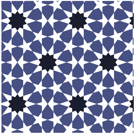
The computational approach involves three phases:
- Construction of a translational unit for tiling the plane
- Constructing a motif for each proto tile which is a part of the translational unit
- Decorating the individual components i.e. new lines and polygons created during motif generation
Patches and Tilings
Let \(\mathcal{T} = \{\mathcal{P_1},\mathcal{P_2} ... \}\)be an infinite collection of polygons. We say that \(\mathcal{T}\) is a tiling of the plane if the polygons in \(\mathcal{T}\) cover the entire plane, leaving no gaps (points that are not covered by any polygon) or overlaps (points that are in the interior of more than one polygon). Here is an example of a tiling of the plane by regular decagons, regular pentagons, and irregular barrel-shaped hexagons.
We define a patch to be a finite collection of nonoverlapping polygons, whose union is a single connected region of the plane with no internal holes.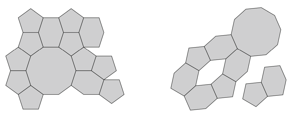
In light of that definition, a tiling might be viewed computationally as a function that consumes regions and produces patches. When two polygonal tiles are adjacent in a patch or tiling, it is possible for a vertex of one polygon to lie somewhere along an edge of the other polygon. We refer to such an arrangement as a T-junction. A patch or tiling will be called corner-to-corner if it contains no T-junctions. When constructing motifs with the polygonal technique we will need to watch out for tilings that are not corner-to-corner.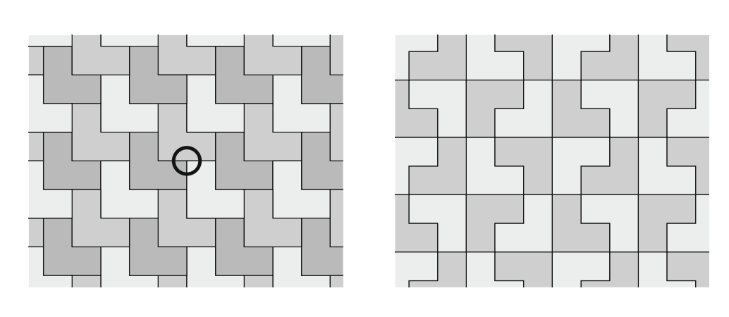
Periodic Tilings
The simple definition of a tiling given above permits tilings with no bound on the complexity of the shapes of the tiles or their arrangement. Periodic tilings, and the broader class of periodic designs to which they belong, play a significant role in ornamental design traditions around the world. Symmetry theory is the standard mathematical tool for characterizing repetition in patterns. A rigid motion in the plane is a symmetry of a given tiling if the transformed tiling lines up precisely with the original, in the sense that every transformed tile lies directly atop some untransformed tile (possibly itself). Note that the identity transformation, which leaves every point in the plane where it is, is a symmetry of every tiling according to this definition; thus every tiling has some nonempty set of symmetries. A tiling is periodic if its symmetries include translations in two nonparallel directions. These translations will necessarily form a two-dimensional family through which the tiling will repeat across the entire plane. For this reason, periodic patterns are also sometimes called wallpaper patterns or all-over patterns.
Periodicity implies a significant amount of redundancy in a tiling, a fact that can readily be exploited in creating software for manipulating periodic tilings. In particular, we can “factor out” all the redundancy, reducing the structure of a periodic tiling down to the following pieces of information:
• A finite patch of tiles, called a translational unit
• Two vectors \(v_1 = (x_1, y_1)\) and \(v_2 = (x_2, y_2)\).
The idea is that the entire tiling can be recovered by assembling transformed copies of the translational unit, translated by vectors \(av_1 + bv_2 = (ax_1 + by_1, ax_2 + by_2)\) for all integers \(a\) and \(b\). For this construction to work seamlessly, the translational unit must be chosen carefully. It must be nonredundant, in the sense that no tile in the patch can be a copy of another tile translated by \(v_1\) or \(v_2\). It must also be maximal, in the sense that enough tiles are included in the translational unit to guarantee that the construction will leave no holes in the plane. (It is not strictly necessary for the translational unit to be contiguous, as is implied by declaring it to be a patch; but it is usually more convenient to choose it as such.) A periodic tiling will typically have many possible translational units, any of which will suffice for the replication process. 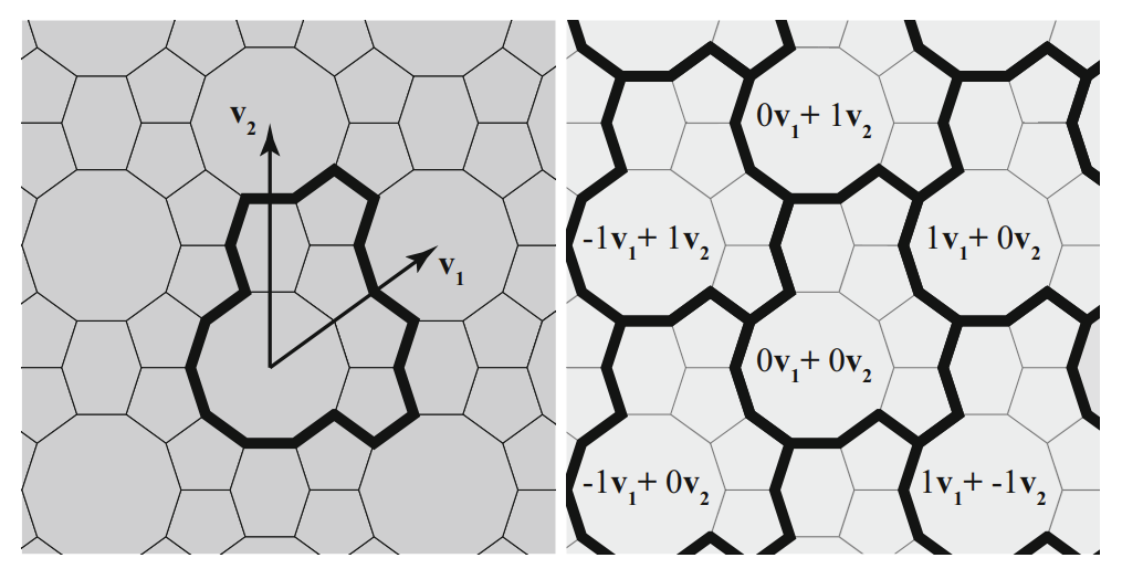
Representation of a translational unit
A translational unit can be represented by the following information:
• An array of \(k\) distinct prototiles, each defined in whatever local coordinate system is most convenient.
• An array of placed prototiles: Each placed prototile is a pair consisting of an index into the array of prototiles, together with a \(3 \times 3\) transformation matrix representing the similarity that transforms the prototile shape to its position in the translational unit.
In this way, whatever procedure we develop for filling tile shapes with motifs, we will need to apply this procedure only once for each unique tile shape. The resulting motifs can be placed in the final pattern using the stored transformation matrices.
Regular and Archimedean Tilings
The simplest tilings of the plane are corner-to-corner tilings by congruent regular polygons, known as regular tilings. It is easy to see that in the Euclidean plane there are only three possible regular tilings, constructed from equilateral triangles, squares, and regular hexagons, as shown below.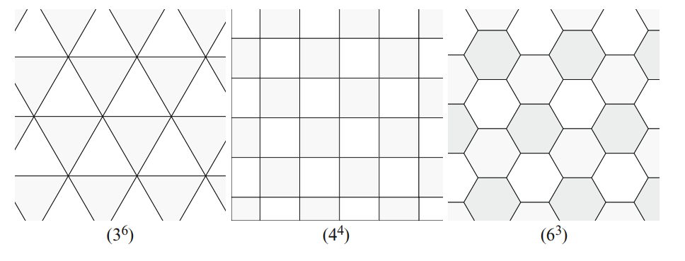
We name each of these tilings using a “word,” consisting of a period-delimited list of the sizes of the polygons encountered around each vertex of the tiling, leading to the names \((3.3.3.3.3.3)\), \((4.4.4.4)\), and \((6.6.6)\), respectively. We use exponentiation for brevity, turning these names into \((3^6), (4^4)\), and \((6^3)\). These tilings appear throughout the world’s decorative traditions, both explicitly and as a basis for more complex design. They will be useful in Islamic geometric design both as underlying polygonal tessellations and as a starting point for constructing other tilings to serve in that role.
If we loosen the constraints above, and consider tilings in which every vertex can be described by a word \(a_1.a_2 \dots a_n\), where each \(a_i\) is an integer greater than \(2\). This generalization introduces eight additional words that can be used at every vertex of a tiling. Canonical tilings exhibiting those words are shown below. These eight, together with the three regular tilings, are known collectively as the semi-regular or Archimedean tilings and are a frequent occurence in Islamic geometric design.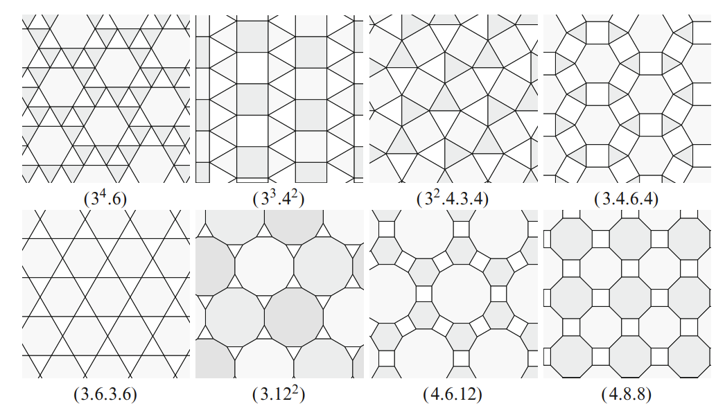
Axis based construction of tilings
This technique is based on identifying points in the plane where regular polygons can be placed, and scaling those polygons so that they link together to define a tiling. Consider the regular tiling \((6^3)\) ), as shown above.
The center of every hexagon in this tiling is the focal point of a collection of symmetries of the tiling. We can rotate the tiling around this point by any multiple of \(60\) and bring it into coincidence with itself. We can also reflect the tiling across six distinct lines through this point, which pass through either the corners or the edge midpoints of the surrounding hexagon. Generally, we refer to any point that acts as the center of a \(360/n\) degree rotational symmetry as an \(n-fold\) axis. The hexagon is only one member of an infinite family of regular polygons that are compatible with all of these symmetries, in the sense that any member of this family can be positioned to map to itself under the given rotations and reflections. If \(m\) is any positive integer, then a regular \(6m\)-gon placed concentrically with the hexagon will share its rotations. Moreover, if we distinguish one ray leaving the hexagon’s center along a line of reflection, then there are two distinct orientations for the \(6m\)-gon that are compatible with the lines of reflection: the ray can pass through either a corner or an edge midpoint. We can therefore represent the choice of polygon to place in this hexagon with two values: an integer multiplier \(m\), and a Boolean indicating whether to place a corner or an edge midpoint on the distinguished ray. The first six combinations of \(m\) and orientation are visualized below. 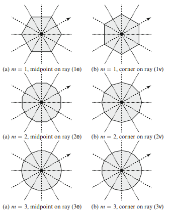
In addition to the sixfold axes at hexagon centers, two other families of rotational symmetries lurk in this tiling: threefold axes at hexagon corners, and twofold axes at edge midpoints. As above, we can choose multipliers and orientations for regular polygons to be centered on these axes.We can visualize this set of choices by constructing a \(30–60–90\) triangle from a hexagon center, the midpoint of an edge of that hexagon, and a vertex of that edge; we call such a triangle a flag. For convenience, we label the \(30^\circ\), \(90^\circ\), and \(60^\circ\) corners \(A\), \(B\), and \(C\), respectively. The polygons described above will be centered at \(A\), \(B\), and \(C\), and we can use the rays \(\overrightarrow{AB},\overrightarrow{BC}\) \(\overrightarrow{CA}\) as a basis for their orientations.
With these labels in place, let \(m_A\), \(m_B\), and \(m_C\) be the integer multipliers for the regular polygons at \(A\), \(B\), and \(C\), and let \(o_A\), \(o_B\), and \(o_C\) be the choices of orientation. We use the letters \(e\) and \(v\) to denote edge and vertex (i.e., corner) orientation; for example, if \(o_A\) is \(e\), then the polygon at \(A\) should intersect the ray \(\overrightarrow{AB}\) at an edge midpoint. The complete arrangement can then be summarized using the notation \([(6^3);m_Ao_A,m_Bo_B,m_Co_C]\). The initial \((6^3)\) indicates that the construction is based on the regular hexagonal tiling.
Any of the multipliers can be zero, indicating that no polygon should be placed on that axis, in which case the orientation can be omitted. This notation does not quite define a tiling, because it fails to provide (up to) three additional numbers: the sizes of the polygons. Because the ultimate goal is to produce a tiling of the plane, it is likely that we will want to scale the polygons until they come into contact with each other.With that in mind,we scale the polygons according to a portfolio of options:
- If only one of the multipliers is nonzero, we scale the single polygon until it comes into contact with the opposite edge of the triangle. For example, in \([(6^3);2e,0,0]\), we would scale the \(12\)-gon at \(A\) until it touches edge \(BC\).
- If two of the multipliers are nonzero, we scale the two polygons until they come into contact with each other. In general, this point of contact can take place anywhere along the flag edge between the two polygons. Usually we add the constraint that the two polygons should have the same edge length, in which case there will be unique radii that bring them into contact. In the context of Islamic geometric patterns, we would like these two polygons to meet with two corners or two edge midpoints on the flag edge.
- If all three multipliers are nonzero, we choose one of the two possibilities. The most direct is based on the previous case: we pick two of the polygons and scale them until they meet and have identical edge lengths, and then scale the third until it touches the nearer of the other two. Or we can scale all three polygons simultaneously until they form a three-way contact. This approach requires solving three equations (which express the fact that the polygons touch) with three unknowns (the sizes of the polygons), suggesting that there will be a unique solution. Of course, we cannot also guarantee in this case that the three polygons will have identical edge lengths. We might therefore produce a non-corner-to-corner tiling.
We can now begin to assemble a translational unit from translated, rotated, and scaled copies of these regular polygons. The translational unit will contain a single copy of the \(A\) polygon if \(m_A \neq 0\), three copies of the \(B\) polygon if \(m_B \neq 0\), and two copies of the \(C\) polygon if \(m_C \neq 0\). Except for a small number of fortuitous cases, the regular polygons will not completely cover the flag, implying that the tiles described so far will leave gaps in the plane. We must therefore introduce additional irregular tiles to fill these holes. The construction given above guarantees that all holes will be congruent copies of a single tile. Depending upon the particular disposition of the regular polygons, the hole filler may span more than one flag, and the translational unit may require \(1, 2, 3, 6\), or \(12\) copies of it. The hole is most easily found by first subtracting the regular polygons from the flag triangle (a standard operation in constructive planar geometry), and then possibly merging multiple copies of the resulting shape into a single larger tile. 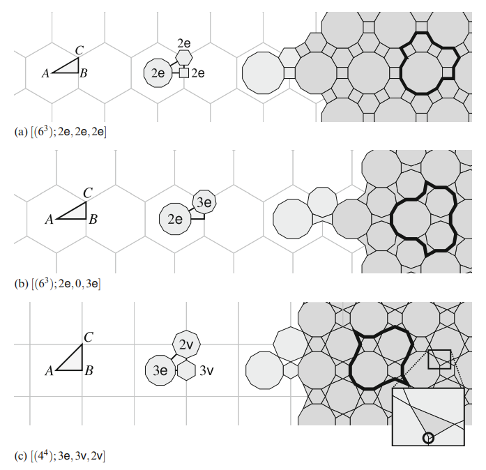
Motifs
Let us assume that we have used the techniques of the previous section to obtain a periodic tiling of the plane based on a small set of regular and irregular polygons. The next step is to produce a line-based motif for each unique tile shape. (We assume for now that we are interested only in the “raw geometry” of the design; the next section will discuss the decoration of Islamic geometric patterns in greater detail.) Once these motifs are constructed, they can be transformed into their final positions to produce a design. The general approach is to choose a contact angle \(θ\) between \(0\) and \(90\), and to construct two rays at the midpoint of each of a tile’s edges. An edge’s rays point towards the interior of the tile, forming two angles of size \(θ\) with the edge. If the corners of the polygonal tile are labeled \(P_1, \dots, P_n\), then we might denote the two rays originating at the midpoint \(M_i\) of \(P_iP_{i+1}\) by \(L_i\) and \(R_i\); the “left ray” \(L_i\) is the one that points to the left of the edge’s perpendicular bisector, and the “right ray” \(R_i\) points to the right. These rays can easily be constructed in software, as shown below.
For example, the origin of \(R_i\) is \(M_i\); the point defining the direction of the ray can be computed by transforming \(P_{i+1}\) by a rotation about this midpoint by angle \(θ\). In a computational setting, it is easy to choose any continuous contact angle between \(0\) and \(90\). The design tradition favors a small set of contact angles based on the geometry of the underlying polygonal tessellation. For example, in the context of the fivefold system, the contact angles for the acute, median, and obtuse families would be \(72^\circ\), \(54^\circ\), and \(36^\circ\), respectively. The key to constructing motifs is to make precise the manner in which these rays encounter rays emanating from other edges, and are truncated into line segments at those meeting points. 
Regular Polygons
Let us assume that we are trying to construct a motif for a regular \(n\)-sided polygon \(P_1, \dots , P_n\). We can further assume that the polygon’s corners lie on a unit circle. A basic motif can always be formed by finding the intersection, for every \(i\), of rays \(R_i\) and \(L_{i+1}\) (with indices taken circularly, so that we intersect \(R_n\) and \(L_1\)). With a bit of trigonometry, we can derive an analytical expression for the locations of these intersections, but in a software implementation it is easier to write a short function that computes the intersection numerically. We can further simplify this process by computing a single intersection this way, and deriving the other \(n-1\) by rotating it around the origin by multiples of \(360/n\) degrees. If we denote by \(C_i\) the intersection of \(R_i\) and \(L_{i+1}\), then the motif will consist of all line segments of the form \(R_iC_i\) and \(C_iL_{i+1}\). This process will fill a regular \(n\)-gon with an \(n\)-pointed star. However, when \(n\) is large and \(θ\) is small, the star will fill the polygon sparsely, producing a design that typically does not have enough visual detail. Traditionally, this deficiency is mitigated by propagating the rays by one extra step, cutting them off at their second intersections rather than their first. This change is equivalent to intersecting \(R_i\) with \(L_{i+2}\) for all \(i\). An easy heuristic is to add this extra layer of geometry whenever \(n \geq 6\).
Two-Point Patterns
The acute, median, and obtuse pattern families use rays that emanate from the midpoints of a tessellation’s polygonal edges. In two-point patterns, the rays grow not from a common origin, but from a pair of points equidistant from the edge’s midpoint. The preceding techniques for regular polygons apply nearly unchanged for two-point patterns. From a given tile edge, construct \(L_i\) and \(R_i\) as before. Then, given a desired separation \(d > 0\), displace \(L_i\) and \(R_i\) by distances \(d/2\) and \(d/2\), respectively, in the direction of the tile edge. That is, compute a unit vector \(\overrightarrow{u}_i\) that points along the edge and add \((d/2)\overrightarrow{u}_i\) to the two points that define the ray \(L_i\) (and similarly for \(R_i\)), as shown.
The remainder of the matching process can proceed as before, except that we do not permit the motif to make use of the correspondence between \(L_i\) and \(R_i\), even though these rays now intersect. We might also need to take this extra intersection into account when decorating the resulting motif. When creating two-point patterns, it is common to set the contact angle to \(45^\circ\), producing squares centered on edge midpoints. Other contact angles can be used as well, in which case rhombs will be produced instead. 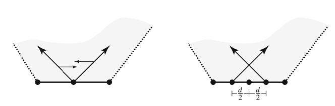
Rosettes
Motifs
When presented with a complex visual stimulus such as an Islamic geometric pattern, the human eye is predisposed to invent an explanation that accounts for that complexity. One way in which this predisposition manifests itself is in the tendency to “chunk” the elements of an ornamental design into larger “super-elements” that appear together. Examining the design below one such superelement demands attention. It consists of a ten-pointed star surrounded by two layers of geometry: a ring of ten kite-shaped quadrilaterals, and a ring of shield-shaped hexagons. The device is known as a rosette.
Rosettes pervade the tradition of Islamic design. There are two ways in which we can take the geometry of rosettes into account as part of a software system for drawing star patterns. The first extends the motif drawing algorithm to construct rosettes within regular polygons; the second intervenes earlier in the pipeline, modifying tilings so that rosettes will arise as they do in the example. A simple method for constructing an \(n\)-pointed rosette within a regular \(n\)-sided polygon is illustrated below. 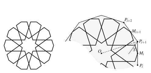
The construction hinges on locating the “shoulder,” labeled \(S\) in the diagram. We can calculate the location of this point by imposing two aesthetically motivated regularity conditions on the rosette. The first is that the outer edges of the shield hexagons align to form (part of) the outline of a regular \(n\)-gon inscribed in the tile. This condition is equivalent to requiring that \(S\) lie on the line \(M_i M_{i+1}\) joining adjacent edge midpoints. The second constraint is that the four outer shield edges have the same length, which we can fulfill by requiring the shoulder to lie on the angle bisector \(\angle OP_{i+1}P_i\) in the diagram. These two constraints are already enough to fix the shoulder position to be the intersection of a line segment and a ray. The remaining constraints on the shape of this rosette follow from requiring the sides of the shield to be parallel to its axis of symmetry.
Dual tiling
In practice, rosettes do not always have the canonical shape suggested above. In particular, the first constraint leaves no flexibility in the rosette’s contact angle, which creates problems when a template tiling contains regular polygons with different numbers of sides. However, it is even better to build the inevitability of rosettes directly into template tilings themselves, in such a way that any compromises that allow them to coexist in a single pattern arise naturally as a consequence of using a single, global contact angle. This transformation is called the “rosette dual,” which begins with a tiling containing abutting regular polygons and produces a new tiling that will lead to the formation of rosettes. The rosette dual behaves similarly to the construction of motifs, in the sense that the goal is to erect a configuration of line segments within each tile of a template tiling. But instead of declaring these “motifs” to be the endpoint of the construction process, they are stitched together to form a new underlying polygonal tessellation. The main step of the rosette dual is then to explain how to construct the necessary configurations within each tile, a process that depends on the kind of tile under consideration. When the tile is a regular \(n\)-sided polygon with \(n \leq 6\), we expect that this polygon will hold the central star within a larger rosette. We fill the tile with a concentric regular \(n\)-gon, rotated so that the corners of the internal polygon point to the edge midpoints of the original tile. The “motif” will be made up of the internal polygon, together with a set of \(n\) radial line segments joining corners and edge midpoints, as shown below. 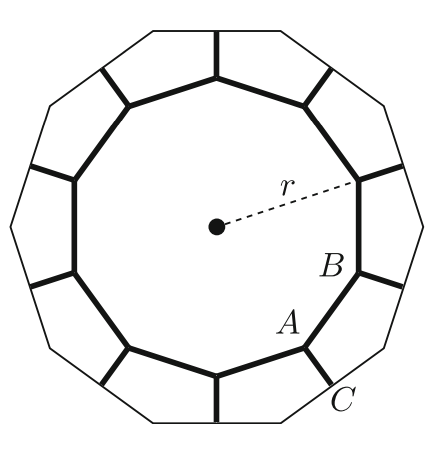
This process is still governed by a free parameter: the radius of the internal \(n\)-gon. We choose this radius so that the internal side length is exactly twice the length of the radial line segments. The rationale is that if a copy of the \(n\)-gon is placed adjacent to this one, the adjacent radial edges in their rosette duals will fuse to create tile edges of the same length as the internal edges.
The preceding per-tile transformations generate a set of planar maps, one for each tile shape. We can assemble multiple transformed copies of these planar maps into a single master planar map, from which the tiles of the rosette dual may be extracted, as illustrated in the figure below. It is necessary to use at least a \(2 \times 2\) grid of translational units, in order to ensure that planar map edges that form partial tiles along the boundary of the translational unit are completed by edges in neighboring units. When the maps corresponding to neighboring tiles are joined, they will leave behind spurious vertices, which lie on the line joining their two neighbors. All such vertices must be spliced out of the master planar map. The faces of the resulting planar map are all tiles of the rosette dual. With a bit of work, we can extract a subset of those faces that make up a translational unit (with the same translation vectors as the original tiling), and group them by congruence so that multiple copies of a single tile shape are encoded correctly.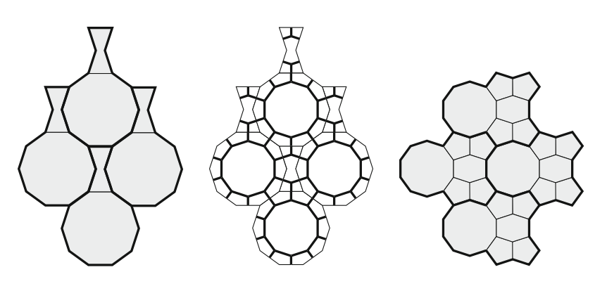
Decoration
The preceding two sections have provided the fundamental building blocks of Islamic star patterns based on the polygonal technique: the template tilings, and the means of elaborating a motif for each different tile shape. These tools are already enough to produce attractive final renderings: take the segments that make up each motif, transform them into position in a translational unit, and stamp out as many units as are needed to fill a region with the pattern.
However, apart from simple schematic drawings, Islamic art is rarely executed in such an abstract manner. Designs are richly decorated in a wide range of styles, media, and colors. Many of those styles are in some sense nonmathematical, being based on floral design or other freeform elements. But there is still a core toolkit of geometric techniques relevant in the production of decorated patterns.
In what follows, it no longer suffices to consider the line segments that make up a motif in isolation; we must understand the complete disposition of vertices, edges, and faces of a motif within a template tile. To that end, let us assume that we have constructed a “tile planar map” for each tile shape, consisting of the polygonal boundary of the tile together with the inscribed motif. In this planar map we will use the terms “boundary edges” and “motif edges” to distinguish the edges originating, respectively, from these two sources.
Filling
The simplest style of decoration is to assign colors to the different regions in a pattern. In practice, we choose a color for each face in a tile planar map, and draw that face as a polygon filled with its corresponding color.Care should be taken to assign colors to boundary faces so that colors are consistent for the faces that share boundary edges.
There is one mathematical feature shared by many of those schemes: frequently, half of the regions are given a single background color, and the other half share a palette of foreground colors. The colors alternate, in the sense no two foreground or background tiles will be adjacent to each other. Mathematically, planar maps for which this sort of coloring is possible are said to be twocolorable. Not every planar map is two-colorable, but barring degenerate cases all the maps constructed as motifs will be. In particular, every vertex in a tile planar map will be the meeting point of either two or four edges, which is a sufficient condition to guarantee two-colorability.
This mathematical fact suggests what could be considered a preliminary step to assist in region coloring: apply a two-coloring to the faces of every tile planar map. We can begin by picking any face containing a boundary vertex and coloring it black; we then perform a depth-first search, walking from a face to its neighbors, coloring white the neighbors of a black face, and vice versa. The example on the right in Fig. 509 shows colored tile motifs that might result from such a process, with some additional color changes applied manually for aesthetic purposes. This algorithm guarantees that like-colored map faces will meet across tile edges when tiles are assembled into a pattern.
Implementation in Python using Numpy
Rhomb tiling and Rosette Dual translation unit
Let us start with the tiling of the plane using rhombs with interior anlges \(72^\circ\) and \(108^\circ\) as shown in the figure. One-quarter of such a rhomb, namely a \(36-54-90\) triangle can function as a flag. Note that \(36\) and \(54\) are both multiples of \(18\), and \(18\) is the angle between adjacent lines of reflection passing through the center of a decagon. In other words, we can place regular \(10m\)-gon around the \(36^\circ\) and \(54^\circ\) angles of this “flag”.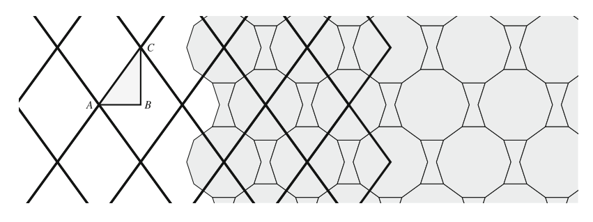
From the above, we get a tiling of the plane where the translational unit consists of regular \(10\)-gon and a bow tie shaped hexagon. Using the rosette dual construction, we end up with a tiling which contains, one regular \(10\)-gon, four pentagons and a barrel shaped hexagon as shown below.
Here is the picture of the translation unit without motifs that will be used for tiling 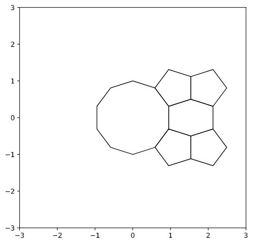
Octagon and square translational unit
In this translation unit, we have an octagon and a square attached to one of the sides with the same side length as that of the octagon.
Here is the picture of the translation unit without motifs that will be used for tiling 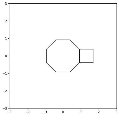
Code for defining the translational units
Each point is defined as numpy array of size \(1\times2\). Each polygon with \(n\) sides is an array of size \(n\times2\). Transformation is defined in terms of a \(3\times3\) matrix which works on homogeneous coordinates.
from math import sin, cos, pi, sqrt
import matplotlib.pyplot as plt
import numpy as np
import matplotlib.patches as patches
from numpy.linalg import inv
from functools import reduce

identity = np.identity(3)

def rotate(angle):
    cosa, sina = cos(angle*2*pi/360), sin(angle*2*pi/360)
    return np.array([[cosa, -sina, 0],
                      [sina,  cosa, 0],
                      [0, 0, 1]])

def shift(tx,ty):
    return np.array([[1, 0, tx],
                     [0, 1, ty],
                     [0, 0, 1]])

def scale(factor):
    return np.array([[factor, 0, 0],
                     [0, factor, 0],
                     [0, 0, 1]])

def regularPolygon(n):
    return np.array([np.array([cos(2*pi*i/n),sin(2*pi*i/n)])
                     for i in range(n)])

def transform(polygon, tm):
    polygon_homo_T = np.hstack([polygon, np.ones((len(polygon),1))]).T

sin18, cos18 = sin(pi/10), cos(pi/10)
sin36, cos36 = sin(pi/5), cos(pi/5)
sin30, cos30 = sin(pi/6), cos(pi/6)
sin54, cos54 = sin(3*pi/10), cos(3*pi/10)

pentagon = regularPolygon(5)
decagon = regularPolygon(10)

def translation_unit1():
    pentagon1tr = reduce(np.dot, [rotate(36), shift(cos18+cos36/(2*cos18),0), scale(1/(2*cos18))])
    pentagon2tr = reduce(np.dot, [shift((cos18+cos36/(2*cos18))*cos36,-(cos18+cos36/(2*cos18))*sin36), rotate(-36), scale(1/(2*cos18))])
    pentagon3tr = reduce(np.dot, [shift(cos18+sin36+cos36/(2*cos18), 2*sin18 + 2*sin18**2), scale(1/(2*cos18))])
    pentagon4tr = reduce(np.dot, [shift(cos18+sin36+cos36/(2*cos18), -2*sin18 - 2*sin18**2), scale(1/(2*cos18))])

    style ={
        "b": {"facecolor":"#475083"},
        "i1": {"facecolor":"#ffffff"},
        "i2": {"facecolor":"#000000"}
    }

    return([(decagon, rotate(18), (72, style)),
            (pentagon, pentagon1tr, (72, style)),
            (barrel_hexagon, np.dot(shift(cos18+sin36,0), rotate(90)), (72, style)),
            (pentagon, pentagon2tr, (72, style)),
            (pentagon, pentagon3tr, (72, style)),
            (pentagon, pentagon4tr, (72, style))
            ],
            np.array([(2+2*sin18)*cos54,(2+2*sin18)*sin54]),
            np.array([(2+2*sin18)*cos54,-(2+2*sin18)*sin54]))

def translation_unit2():
    pentagon1tr = reduce(np.dot, [rotate(36),shift(cos18+cos36/(2*cos18),0),scale(1/(2*cos18))])
    pentagon2tr = reduce(np.dot, [shift((cos18+cos36/(2*cos18))*cos36,-(cos18+cos36/(2*cos18))*sin36),rotate(-36), scale(1/(2*cos18))])
    pentagon3tr = reduce(np.dot, [shift(cos18+sin36+cos36/(2*cos18), 2*sin18 + 2*sin18**2),scale(1/(2*cos18))])
    pentagon4tr = reduce(np.dot, [shift(cos18+sin36+cos36/(2*cos18), -2*sin18 - 2*sin18**2),scale(1/(2*cos18))])

    style1 ={
        "b": {"facecolor":"#ffffff"},
        "i1": {"facecolor":"gray"},
        "i2": {"facecolor":"#ffffff"}
    }

    style2 ={
        "b": {"facecolor":"#ffffff"},
        "i1": {"facecolor":"gray"},
    }

    return([(decagon, rotate(18), (72, style1)),
            (pentagon, pentagon1tr, (72, style2)),
            (barrel_hexagon, np.dot(shift(cos18+sin36,0), rotate(90)), (72, style2)),
            (pentagon, pentagon2tr, (72, style2)),
            (pentagon, pentagon3tr, (72, style2)),
            (pentagon, pentagon4tr, (72, style2))],
            np.array([(2+2*sin18)*cos54,(2+2*sin18)*sin54]),
            np.array([(2+2*sin18)*cos54,-(2+2*sin18)*sin54]))

def translation_unit3():
    squaretr = reduce(np.dot, [shift(cos22_5+sin22_5,0),rotate(45),scale(2*sin22_5/sqrt(2))])
    style1 ={
        "b": {"facecolor":"#d9cbb4","linewidth":0.5, "edgecolor":"black"},
        "i1": {"facecolor":"#58a0cd","linewidth":1, "edgecolor":"black"},
        "i2": {"facecolor":"#d9cbb4","linewidth":1, "edgecolor":"black"}
    }

    style2 ={
        "b": {"facecolor":"#d9cbb4"},
        "i1": {"facecolor":"#58a0cd", "linewidth":1,"edgecolor":"black"},
    }

    return([(octagon, rotate(22.5), (72, style1)),
            (square, squaretr, (72, style2))],
            np.array([2*cos22_5*cos45,2*cos22_5*sin45]),
            np.array([2*cos22_5*cos45,-2*cos22_5*sin45]))
Code for creating the motifs
The function below, takes a polygon as input and returns a list of polygons that are the result of tesselation of the original polygon after creating the motif. Each polygon is identified as an interior polygon or a boundary polygon (I am cutting corners here instead of creating a proper planar map using a data structure like a doubly connected edge list).
In case the polygon has greater than \(6\) sides, we have one innermost interior polygon and another set of interior polygons with a vertex on the boundary adjacent to the innermost interior polygon.
def motif(polygon, angle):
polygons = []
n = len(polygon)
cosa, sina = cos(angle*2*pi/360), sin(angle*2*pi/360)
M, L, R = [], [], []
for i in range(n):
m_x, m_y = 0.5*(polygon[i] + polygon[(i+1)%n])
r_x,r_y,_ = reduce(np.dot, [shift(m_x,m_y), rotate(angle), shift(-m_x, -m_y),
np.array([polygon[(i+1)%n][0], polygon[(i+1)%n][1],1]).T])
l_x,l_y,_ = reduce(np.dot, [shift(m_x,m_y), rotate(-angle), shift(-m_x, -m_y),
np.array([polygon[(i+1)%n][0], polygon[(i+1)%n][1],1]).T])
M.append(np.array([m_x, m_y]))
L.append(np.array([l_x, l_y]))
R.append(np.array([r_x, r_y]))
IP1, IP2 = [], []
for i in range(n):
t1,_ = np.dot(inv(np.array([R[i] - M[i],M[(i+1) % n] - L[(i+1) % n]]).T),
(M[(i+1) % n]-M[i]).T)
IP1.append(M[i] + t1*(R[i]-M[i]))
if n > 6:
t2,_ = np.dot(inv(np.array([R[i] - M[i],M[(i+2) % n] - L[(i+2) % n]]).T),
(M[(i+2) % n]-M[i]).T)
IP2.append(M[i] + t2*(R[i]-M[i]))
int_polygon = []
if n<=6:
for i in range(n):
int_polygon += [M[i], IP1[i]]
polygons.append((np.array([M[i], polygon[(i+1)%n], M[(i+1)%n], IP1[i]]),"b"))
polygons.append((np.array(int_polygon),"i1"))
else:
for i in range(n):
int_polygon += [IP1[i], IP2[i]]
polygons.append((np.array([M[i], IP1[(i-1)%n], IP2[(i-1)%n], IP1[i]]),"i1"))
polygons.append((np.array([M[i], polygon[(i+1)%n], M[(i+1)%n], IP1[i]]),"b"))
polygons.append((np.array(int_polygon),"i2"))
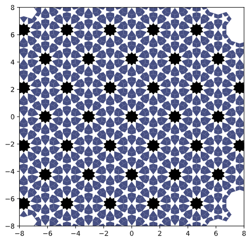
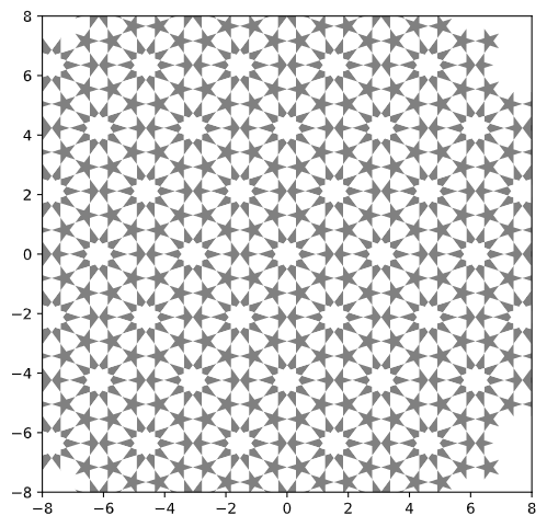
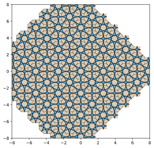
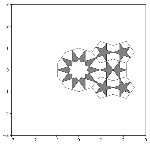
return polygonsHere are the pictures of the same translational units with different decoration styles using the same motif 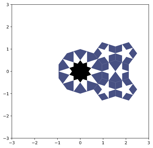

Code for plotting the tiling
def plot_polygons(axes, polygons, styles=None, style_default={"facecolor":"None","linewidth":1,"edgecolor":"black"}):
    for i, p in enumerate(polygons):
        if not styles:
            poly = patches.Polygon(p, **style_default)
        else:
            poly = patches.Polygon(p, **styles[i])
        poly.set_transform(axes.transData)
        axes.add_patch(poly)
    return axes

def plot_translation_units(axes, translation_unit, tiling_pos=[(0,0)], show_motif=False):
    polygons_transforms, v1, v2 = translation_unit
    polygons, styles = [], []
    for i,j in tiling_pos:
        shiftx, shifty  = i*v1 + j*v2
        shift = [[1,0,shiftx],[0,1,shifty],[0,0,1]]
        for polygon, tr, (angle, style) in polygons_transforms:
            if not show_motif:
                polygons.append(transform(transform(polygon,tr), shift))
            else:
                for p, ty in motif(polygon, angle):
                    polygons.append(transform(transform(p,tr), shift))
                    styles.append(style[ty])
    plot_polygons(axes, polygons, styles)

plt.figure(figsize=(6,6))
axes = plt.gca()
axes.set_xlim([-8,8])
axes.set_ylim([-8,8])
tiling_pos=[(i,j) for i in range(-4,4) for j in range(-4,4)]
plot_translation_units(axes, translation_unit1(), tiling_pos, show_motif=True)
Here are the pictures of the tiling generated using the translational units defined above